Document classification: Classifying contract types

In this tutorial, you will be using Snorkel Flow to train and build a model that will classify 20,000+ SEC filings into one of the four following types: employment, services, stock, and loan. Thanks to the programmatic labeling available in Snorkel Flow, you will be able to label your training data using Labeling Functions, train your models, and view an analysis that will guide you through an iterative development process - a new way of building AI applications!

This tutorial is intended for first-time users of Snorkel Flow who are very new to the data-centric AI, programmatic labeling and machine learning models.

What you will learn in this tutorial:

• Application setup
  • Uploading data into Snorkel Flow
  • Creating a new application
• Snorkel Flow Model Suite overview
  • Create Labeling Functions (LFs): programmatically label your data
  • Train a Machine Learning (ML) model: generalize beyond your LFs
  • Analyze model errors and results: identify model errors and improve model results

Application setup

Uploading data

When you open Snorkel Flow, you will be on the Applications page. Before you create your first application, you will first need to upload some data. We begin by creating a new dataset in your instance.

To do this:

• Click the Datasets option from the left menu
• Click the + New dataset button on the top right corner of your screen

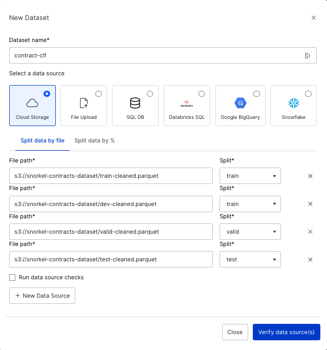
You will be brought to our New Dataset page below. Data can be ingested into Snorkel Flow from a range of storage options including cloud storage, databases or local files. For this tutorial, we provide an example dataset that is saved in AWS S3 Cloud Storage. The table below contains the 4 files we will be uploading to this dataset.

Data source	File path	Split
1	s3://snorkel-contracts-dataset/train-cleaned.parquet	train
2	s3://snorkel-contracts-dataset/dev-cleaned.parquet	train
3	s3://snorkel-contracts-dataset/valid-cleaned.parquet	valid
4	s3://snorkel-contracts-dataset/test-cleaned.parquet	test

Fill in the New Dataset page with the following information:

• Give it the name contract-clf
• Ensure that you are selecting Cloud storage as your data source.
• Under Split data by file, add a data source for each of the 4 data sources listed in the table above.

Your New Dataset page should now look like this:

We've uploaded 4 different data splits for our application, each with a specific purpose for model development:

• Train: The initial training dataset that is used to develop your machine learning model. The train split does not need to have any labels. This tutorial however, has included a small number of them so that you can look at them during development to get an idea of the classification problem (see description of the dev split below). This tutorial walks through how to build consistent labels in the data in your train split.

• Dev: The dataset that is used for development of Labeling Functions. This is the dataset viewable inside the model suite, and is randomly sampled from the train split. The application suite shows the dev split over the entire training dataset to limit the amount of data in memory. By default, 10% of the train split, up to 2000 samples, is used for the dev split.

• Test: The ground truth that is held-out from the training dataset for evaluation purposes. While not strictly necessary, it is recommended to use as a final evaluation against ground truth (i.e. expert annotated) labels.

  note

  You should not look at any of these data points, or else you risk biasing your evaluation procedure!

• Valid: Similar to test, the valid split contains some ground truth labels for evaluation purposes. This split can be used to tune your ML model.

Once all information above is added, you can click Verify data source(s) to run data quality checks to ensure data is cleaned and ready to upload.

After clicking Add data source(s), you will see a UID column drop-down box. Select uid, which is the unique entry ID column in the data sources, and again click Add data source(s) to continue.

When the data is done ingesting on all four data sources, you are ready to move on to the next step!

For more information about uploading data, see Data upload.

Creating an application

Now that our data is uploaded to our application, we will create a new Application to make use of our dataset. To create a new application:

• Click the Applications option in the left-side menu.
• Click the drop-down arrow on the Create application button (top right corner of your screen), then click Create from template.

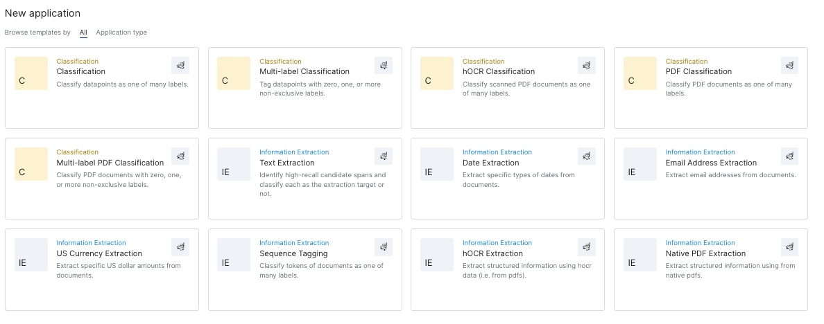
This will bring you to our existing list of pre-set application templates, with a template page similar to the image below. These are starter templates to help solve a variety of different machine learning problems and tasks. For our specific task, we will need a Classification application that will create an application to label entire documents across our desired schema. Click the Classification template on the top left of your screen, then click Create application in the next pop-up.

After choosing your application template, the New Classification application screen will ask for various information to help populate our new application. This page helps us set up your desired application correctly. Please enter the following information for each option:

Option	Value
Application name	cls-contract
Choose default dataset	contract-clf
Specify required input fields	text (leave all other options unchecked)
Ground truth column (Optional)	label

After inputting this information, click Autofill Labels to populate your labeling schema into the Labels (optional) field based on existing data in your label column. Your New Classification application template should look like the below image:

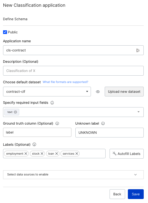
Click Save to initiate application creation. This will take anywhere between 2-5 minutes, as Snorkel Flow starts ingesting your data into the existing application template and prepares the data for programmatic labeling.

Snorkel Flow model suite overview

Once the application is prepared, you should be brought to our Studio page. We are now ready to start developing a model in your new application! The remainder of this guide will cover the 3 key aspects of programmatic labeling:

1. Developing Labeling Functions (LFs)
2. Train a Machine Learning (ML) Model
3. Analyze model results

Developing labeling functions (LFs)

We will begin creating Labeling Functions (LFs) that best label our data according to their existing criteria. LFs are the "programmatic" labeling piece in Snorkel Flow. Using LFs, we codify expert opinion and criteria for how to label our data. These labeled data points help create more training data and achieve better model results.

Filtering data

For our first LF, we will first focus on developing a highly precise LF for employment contracts. We will start by filtering our data for only documents that are labeled employment. To do this:

• Click the Filter icon at the top right corner of your screen.
• Click Ground Truth.
• Choose Ground Truth -> is -> employment from the drop-down menu

You should have a screen similar to the attachment below:

Finally, click the checkmark and this will filter viewable data to only be employment documents.

Changing the data viewer

We can also change how you view your data in the platform. On the middle left of your screen, the data defaults to Record view. Click on this to see a drop-down of several data viewing options:

• Record view shows all columns for a single article.
• Snippet view shows small snippets of text for all articles.
• Table view shows all columns for all articles, similar in format to an Excel sheet.

For this exercise, select Table or Snippet view to look at several documents at the same time.

Creating your first LF

As you scan across the various employment articles, you will start to see an emerging pattern. Most employment documents start with EMPLOYMENT AGREEMENT. Let's create our first LF that labels all documents containing EMPLOYMENT AGREEMENT as employment.

To create our LF, navigate to the top middle pane of the UI with the description Type anything to start creating your LF. Type an / into the field, and click Keyword under the Pattern Based section. This should bring up the following segment:

Then do the following:

• Add "EMPLOYMENT AGREEMENT" (including the double quotes) into the Keywords space.
• Click Select a label on the right side of the LF builder, and then select employment.
• Finally, click Preview LF.

The UI is updated to provide several metrics on the quality of the LF that appear inside of the LF builder:

• Prec. (GT) measures the precision of the LF on your current data split (i.e., a measure of how often the LF correctly labels the documents based on the ground truth).
• Coverage details the % data in your split that fit this criteria.

The data in your UI is also filtered to only show documents fitting this criteria.

This LF has 93.6% precision and 32.4% coverage, which is highly accurate. Click Create LF to add it to your active LFs. You can use the Labeling Functions side bar to help manage your active LFs.

LF best practices and tips

There are a variety of different types of LFs at your disposal in the platform. Please iterate and try several types of LF builders that will best label your current data.

As you continue iterating and building LFs, we recommend the following:

• Shoot for High precision and low coverage LFs. This will ensure that the LFs will provide labels for our ML model with high accuracy. To help achieve high precision results, consider including additional criteria into your existing LFs. For example, we can incorporate a second criteria to our previously created Employment Agreement LF that also excludes all documents that mention purchase.

• Build several LFs for each label in your model to ensure adequate LF coverage of your training data.
  • Click View LF coverage under the Labeling Functions side bar to keep track the label functions for your ground truth data points. This will show a drop down similar to the below image that details the LF coverage of the ground truth, and shows which labels are lacking LF coverage.

• • You can track total LF coverage of your current data split on the top left of your screen. Choose LF coverage from the drop-down to see the total % data points with LF labels in your dataset. under LF coverage. You can also choose LF conflict to see the total % data points that have LFs with conflicting values.
• Your LFs do not need to be perfect in terms of accuracy and coverage. Snorkel Flow will use an ML model to generalize beyond and correct incorrect outputs from the LFs. However, improving the accuracy of the LFs will almost always result in higher model performance. The Analysis side bar will show which LFs need additional improvement.

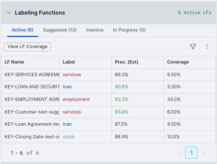
For now, we provide the following keyword LFs to help you build additional high-precision LFs and increase the LF coverage of your dataset:

LF Type	Keywords	Label
Keyword	"SERVICES AGREEMENT"	services
Keyword	"LOAN AND SECURITY AGREEMENT"	loan
Keyword	"Closing Date"	stock
Keyword	"Customer"	services
Keyword	"Loan Agreement"	loan

Build these LFs following the same steps that you took to create the "EMPLOYMENT ASSESSMENT" LF. Once you've created each of these LFs, you will see the 6 active LFs in the Labeling Functions side bar on the left side of your screen. Note that your values may look different than what is presented in this screenshot.

Train a machine learning (ML) model

Now that we've created several LFs for our model, we are ready to train our first ML model! We will try various ML models and test the predictability of our current dataset. This will be the most important aspect of our tool, as the final model results determine success for our current application. Our main goal will be to achieve at least 90 accuracy and 90 F1 for our Valid data split. We will provide details for running a Fast model below.

To run your first ML model, go to the Models side bar on the left and click Train a model. This will bring us to the 3 different ML model training options: Custom model, Fast model, or AutoML. We will first run a Fast model as this model runs significantly faster than the other options. It runs only a subset of the training data through the model and provides a good starting baseline for our model results. Select Fast model, then click Train Fast Model to officially kick-off model training for our dataset.

Once model training is kicked off, a status bar appears that shows the model training progress. This will provide a % of model training completion.

Once the model is finished training, it will update the table attached to the Models side bar with the most recent model metrics.

So far, the results are a good start but are still below are desired 90 Accuracy and 90 F1 success metrics. We will now visit the Analysis side bar to identify which data points and labels our model struggles to predict.

Analyze model errors and results

After running the first ML model, you can view the model in the Analysis side bar. We will discuss the 2 most common error analysis visualization tools in the platform, but we strongly recommend utilizing the other analysis tools along with these to best identify the source of errors in your model.

Clarity matrix

The Analysis side bar automatically shows the Clarity matrix by default. The table below shows where our model incorrectly predicts outputs from our LFs, and whether incorrect model outputs came from LFs that were incorrect, correct, or low confidence (i.e., data points not covered by our LFs). This table is particularly helpful for understanding how we can improve our current model results; for each incorrect model output, we have defined next steps for model improvement.

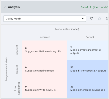
Filters are applied to our existing UI data when you click the Refine existing LFs and Write new LFs boxes. This helps to identify the specific data points that fall into these buckets.

Confusion matrix

We also provide a Confusion matrix to view the errors between the different labels in your model results. To view this, select Confusion matrix from the drop-down menu. The counts on the diagonal represent correct predictions, and the off-diagonal counts represent errors in the model results. We can see specifically which classes the model predicts incorrectly, as well as the ground truth associated with those classes. Similar to the Clarity matrix, clicking any of the red buckets will filter the data in our UI by data points falling into each of those buckets.

For additional insight into different model analysis techniques and how to improve model performance, see Analysis: Rinse and repeat.

Next steps: Iterate

At this point, you are well versed with the most common features and capabilities of the Snorkel Flow platform and are ready to work towards achieving our success metrics! See if you can improve the model performance for this dataset and task by using the Analysis visualizations to tweak your LFs and models for better results. In this way, improving (and adapting) your model becomes a fast, iterative, and error analysis-driven process in Snorkel Flow rather than a slow and ad hoc one blocked on hand-labeled training data.

As you continue to iterate on your results, we recommend utilizing the below additional features:

• Custom model in our Models pane
• Search based LFs