Image Studio reference

This page walks through the key components of using Image Studio for your image classification applications:

• Prerequisites to get started
• Exploring your data
• Annotating your data
• Creating labeling functions
• Training models
• Exporting your data

Prerequisite: Enable dedicated resources

Because image data is large and computationally expensive, you must first enable dedicated resources on your application before developing labeling functions (LFs) and models. Snorkel Flow will then allocate compute resources so that you have faster and more performant backend operations on much larger dataset sizes. This allows you to scale up to 500K data points in a split sample. For step-by-step instructions on how to enable dedicated resources on your application, see Using dedicated resources to speed up applications with large datasets.

note

Snorkel may take time to cache the dataset upon initial load.

note

When you are finished, be sure to de-allocate dedicated resources to free up memory for others to use.

Explore your data

Image Studio provides three views from which you can explore your data:

• Grid: View multiple images in a gallery view.
• Image: View an individual image and its associated metadata.
• Data: View image data along-side any text-based metadata.

The following sections walk through the available views in more detail.

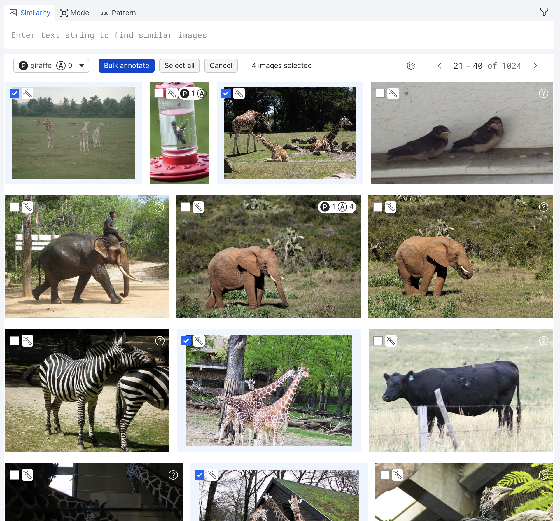
Grid view

Grid view allows you to view multiple images at a time in an elegant photo gallery view. This provides you with a broad overview of what the images in your dataset look like.

You can also annotate ground truth in Grid view. See Annotate your data for more information.

Click the gear icon customize the view settings:

• Page size: Specify how many images are viewable per page.
• Export Studio dataset: Export your dataset into a CSV file. You can specify what columns to export as well as which model to include predictions from.
• Resample data: Opens a modal with various resampling options:
  • Sample size: The approximate number of data points to sample from a split.
  • Max labeled: The maximum number of labeled data points to include in the sample.
  • Min per class: The minimum number of data points per class to include in the sample.
  • Random seed: A random integer seed to use for deterministic sampling.

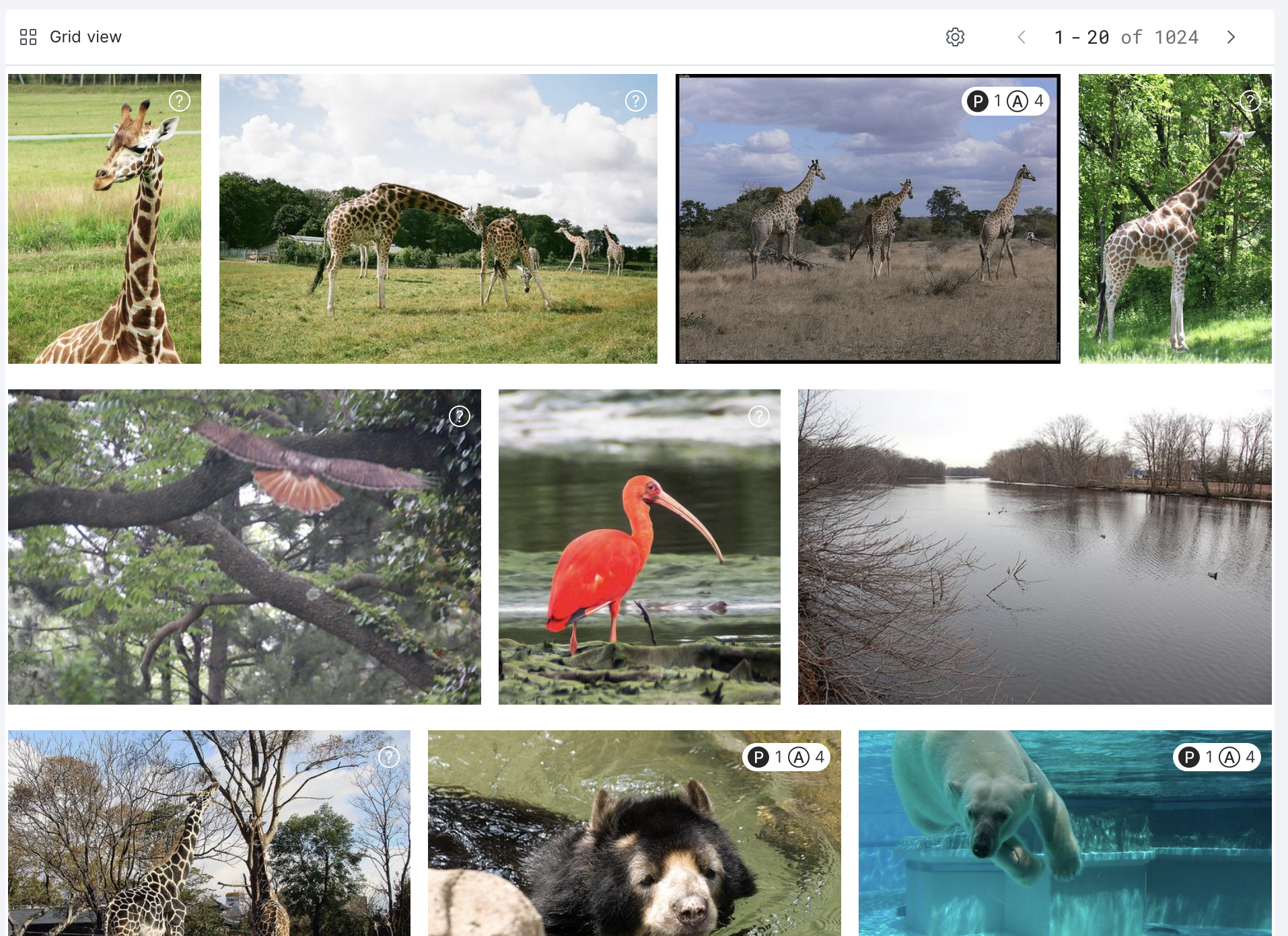
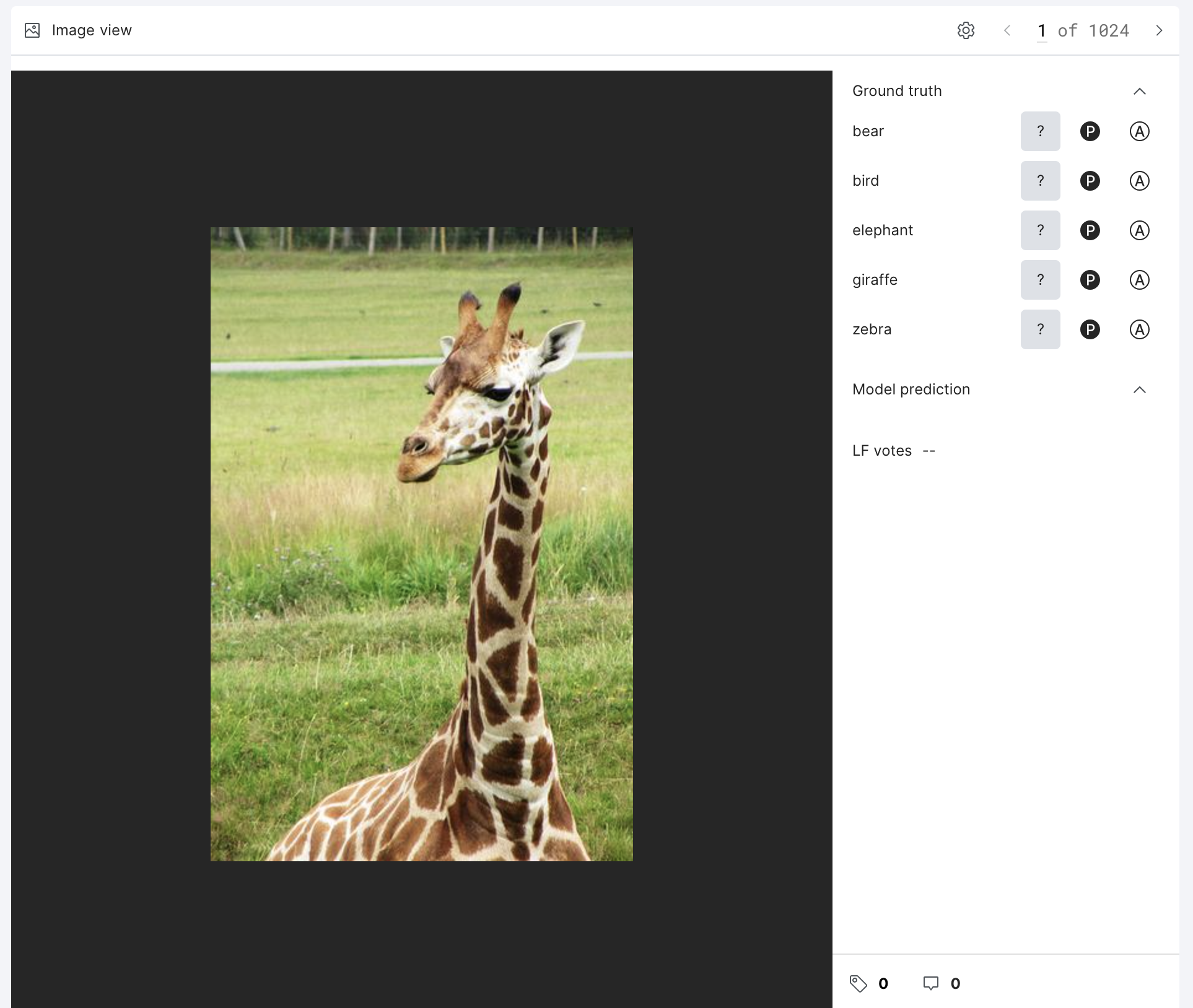
Image view

If you are paging through images in Grid view, and want a more detailed view of an individual image, select that image to open it up in Image view. Here, you can view an individual image and its associated metadata. You can view an image's ground truth, model predictions for the selected model, LF votes, and have access to tags and comments. In addition, you can update the ground truth of the image.

Click the gear icon customize the view settings:

• Export Studio dataset: Export your dataset into a CSV file. You can specify what columns to export as well as which model to include predictions from.
• Resample data: Opens a modal with various resampling options:
  • Sample size: The approximate number of data points to sample from a split.
  • Max labeled: The maximum number of labeled data points to include in the sample.
  • Min per class: The minimum number of data points per class to include in the sample.
  • Random seed: A random integer seed to use for deterministic sampling.

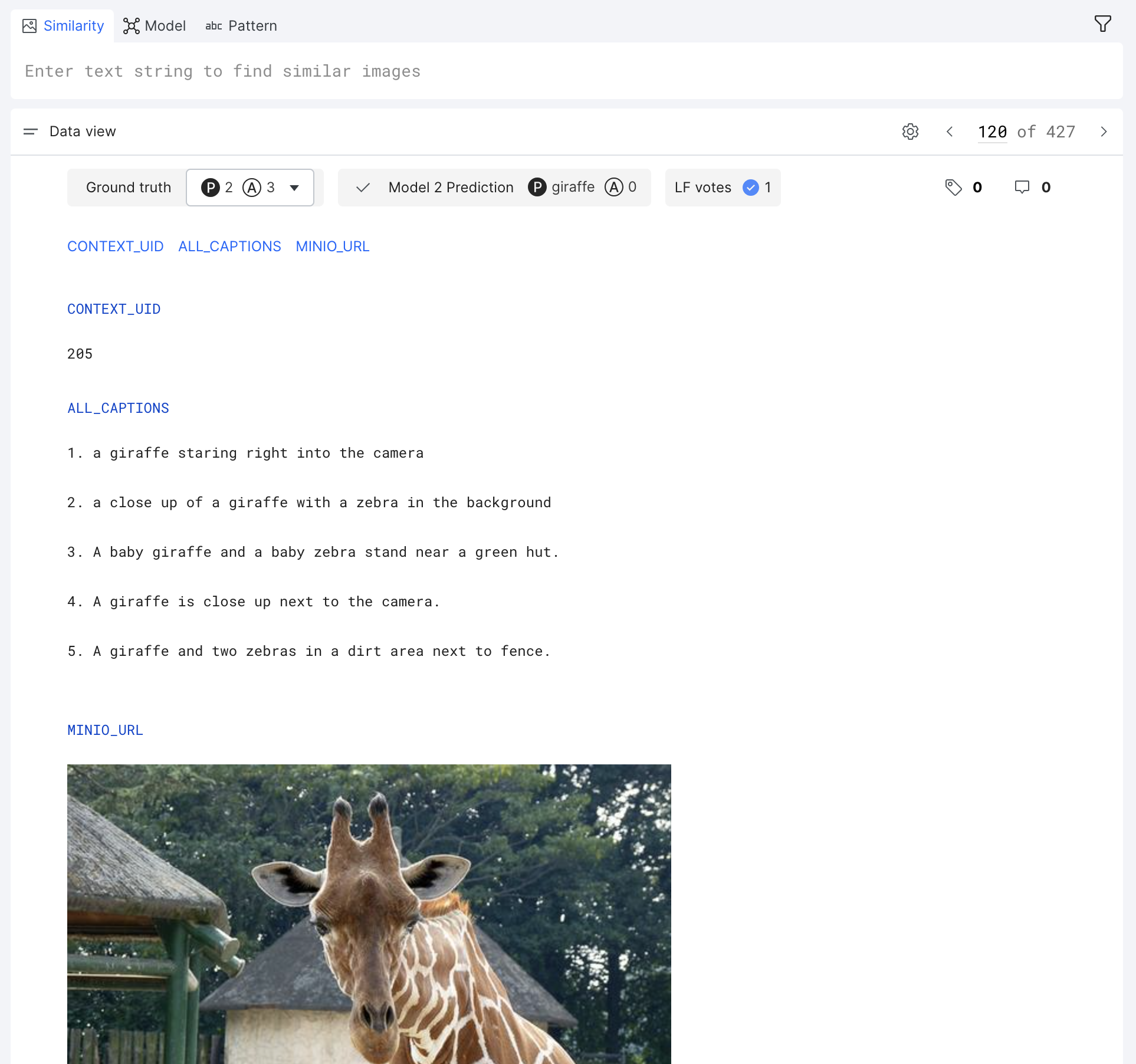
Data view

Data view allows you to view image data alongside any text-based metadata, such as captions. This is particularly useful for writing LFs based on pattern matches against text columns.

Click the gear icon customize the view settings:

• Select displayed fields: Customize the data fields that are displayed.
• Export Studio dataset: Export your dataset into a CSV file. You can specify what columns to export as well as which model to include predictions from.
• Resample data: Opens a modal with various resampling options:
  • Sample size: The approximate number of data points to sample from a split.
  • Max labeled: The maximum number of labeled data points to include in the sample.
  • Min per class: The minimum number of data points per class to include in the sample.
  • Random seed: A random integer seed to use for deterministic sampling.

Annotate your data

Image Studio supports simple ground truth annotation workflows to easily annotate your data from any data view. Images can be labeled with multiple classes by three statuses: Present, Absent, or Abstain.

Grid view supports a special bulk annotation feature that allows you to label multiple data points at the same time. Use this to easily apply class labels to batches of image data points.

Create labeling functions (LFs)

Labeling functions (LFs) are programmatic rules or heuristics that assigns labels to unlabeled data without the need for manual annotations. Each labeling function is defined for a single class such that it votes whether or not the image should be assigned to that class. See Introduction to labeling functions (LFs) for more information.

There are three types of LFs that can be generated in Image Studio:

• Similarity: Labels images based on their similarity score to text, other images, or cropped images.
• Model: Labels images based on the model predictions of a pre-trained model.
• Pattern: Labels images based on user-defined rules (e.g., keyword or regex match) against text data that is associated with your images. This is a native feature in Snorkel Flow.

The following sections walk through the available LFs in more detail.

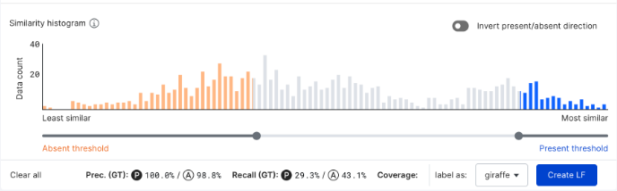
Similarity histogram

Each LF tool includes a visual similarity histogram that you can use to filter the data points that you would like to label. The histogram ranks your data points from left-to-right as least similar to most similar. That is, the selector on the left selects data points with low similarity scores that will be labeled as absent. Similarly, the selector on the right selects data points with high similarity scores that will labeled as present. All unselected images are not labeled (i.e., are abstained).

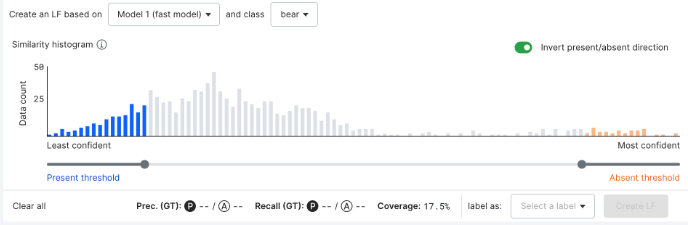
You can turn on the Invert present/absent direction option to incorporate simple negation into your LFs. When the LF is inverted, data points that are selected as least similar on the left will be voted as present, while data points that are selected as most similar on the right will be voted as absent.

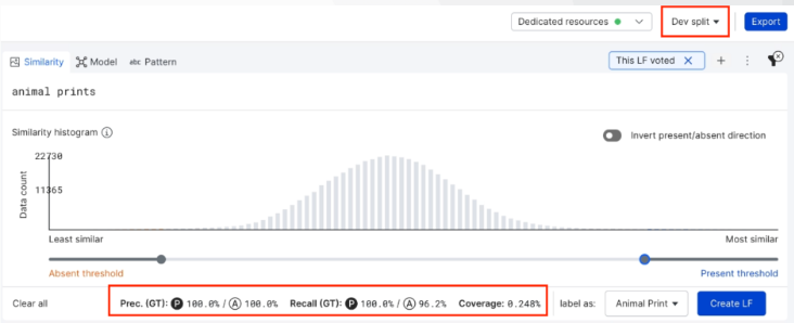
As you adjust the thresholds, the precision and recall values for predicting both present and absent labels are automatically updated for the current split. This is usually the dev or train split rather than the valid split. Because of this, we recommend adding a small sample of ground truth labels for each into in to the dev/train splits, in addition to keeping the majority of ground truth labels within the valid split.

Similarity LFs

There are three types of similarity LFs that you can create:

LF	Input	Output
Image-to-text comparator	Text query	OpenAI CLIP similarity score
Image-to-image comparator	Dataset image	OpenAI CLIP similarity score
Image-to-image patch comparator	Cropped dataset image	OpenAI CLIP similarity score

Image-to-text comparator

The text-to-image comparator LF tool accepts a text query and outputs image matches ranked by their embedding similarity score. These embeddings are computed using the OpenAI CLIP model.

To create an image-to-text LF:

1. Select the Similarity tab on the LF composer toolbar.
2. In the textbox, write a text string for which you would like to find similar images.
3. Click Preview LF.
4. Select the class that you want to label in the label as drop down.
5. Use the similarity histogram to adjust the thresholds for the images that you would like to label with this LF.
6. Once you are happy with the thresholds that you have selected, click Create LF.

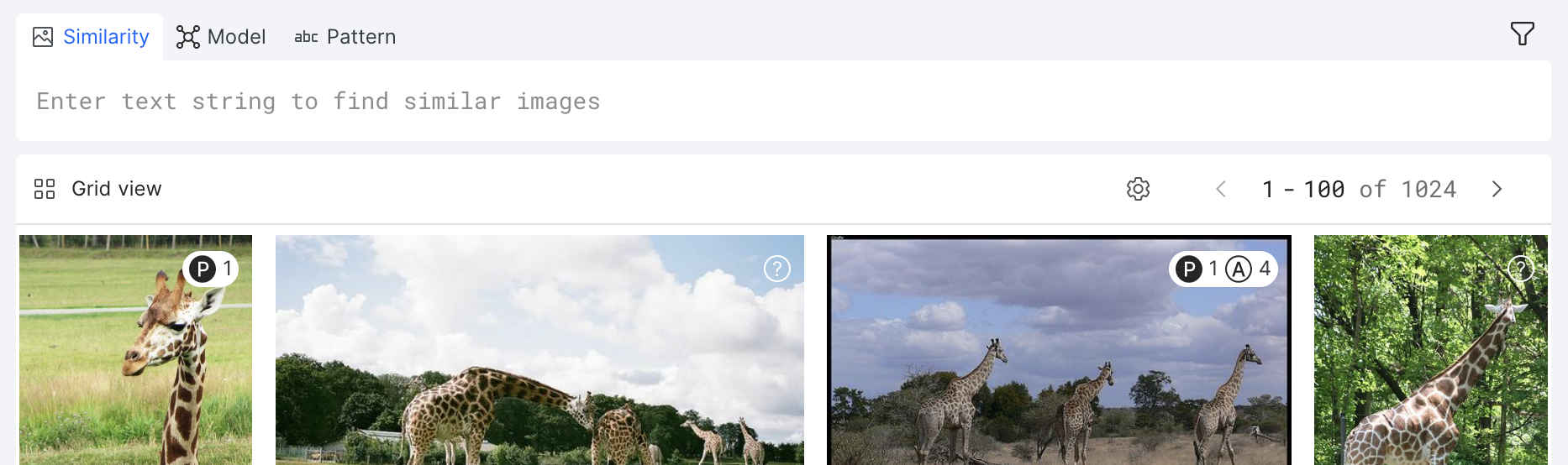
Image-to-image comparator

The image-to-image comparator LF tool allows you to select any image using the magic wand tool and outputs image matches ranked by their embedding similarity score. These embeddings are computed using the OpenAI CLIP model.

To create an image-to-image LF:

1. Select the Similarity tab on the LF composer toolbar.
2. Select the image that you want to perform a similarity search.
   • In Grid view, hover over the image, and then select the magic wand button.
   • In Image view, hover over the image, and then click Preview image LF.
3. Select the class that you want to label in the label as drop down.
4. Use the similarity histogram to adjust the thresholds for the images that you would like to label with this LF.
5. Once you are happy with the thresholds that you have selected, click Create LF.

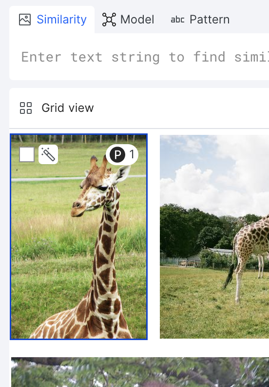
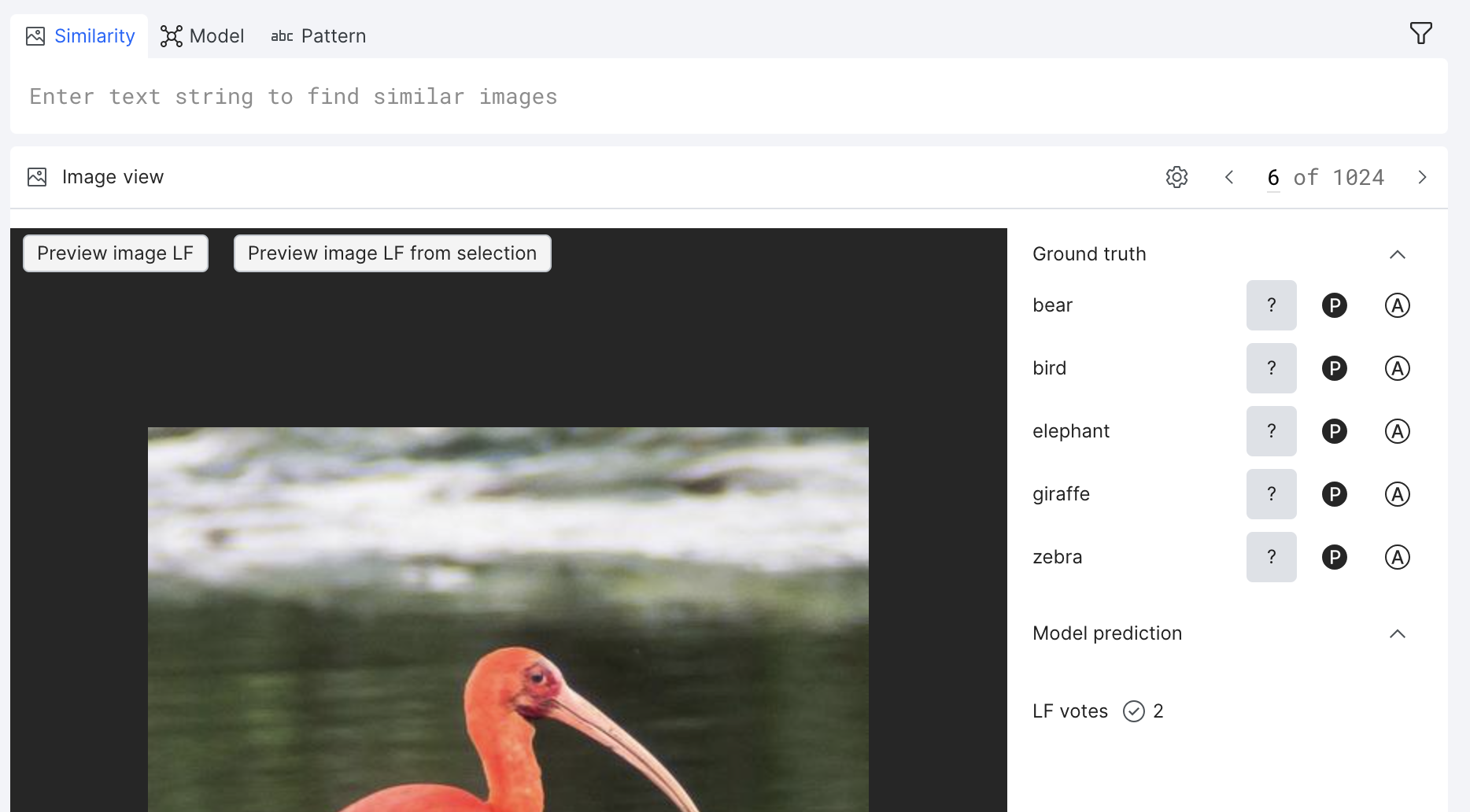
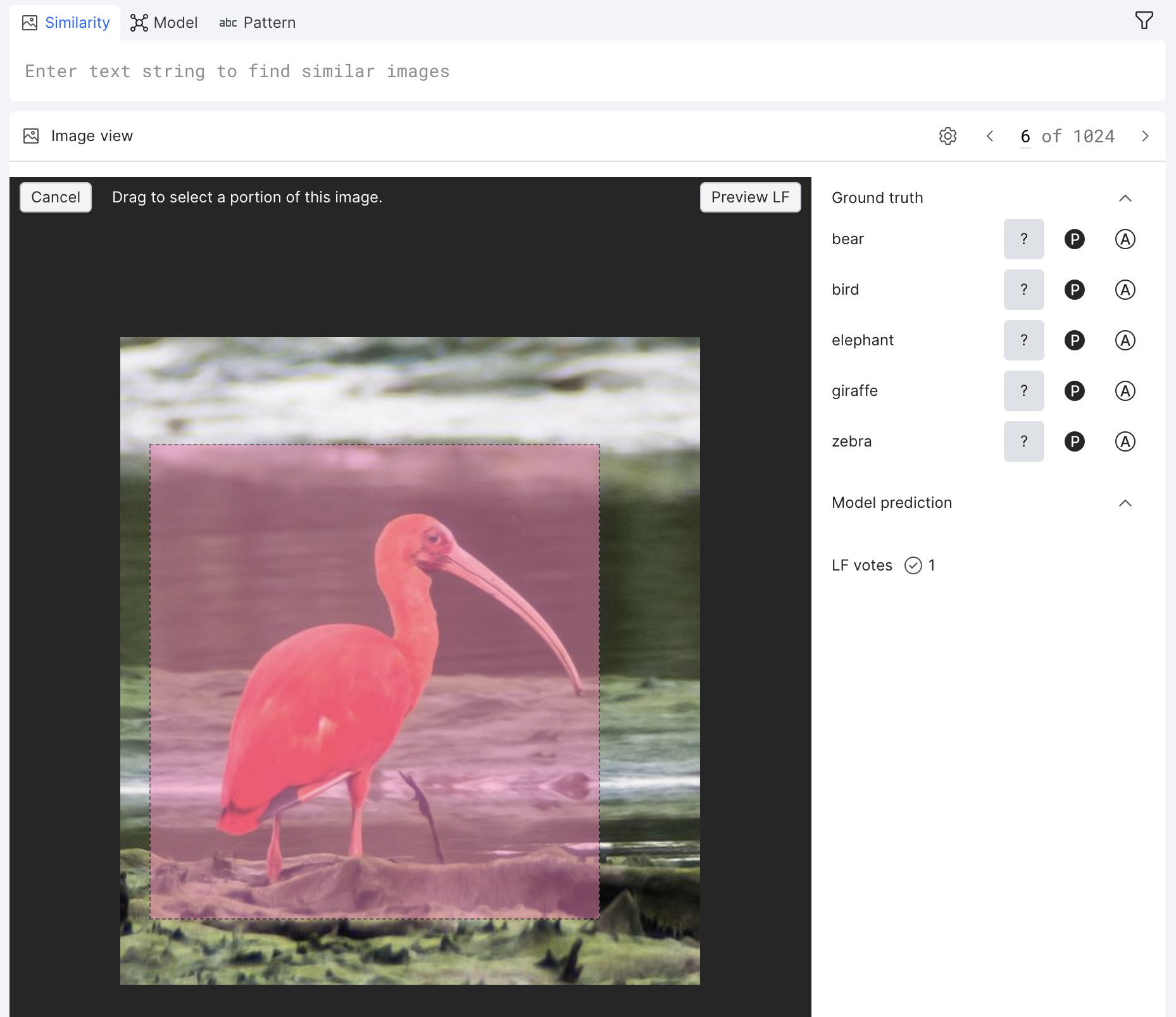
Image-to-image patch comparator

The image-to-image patch comparator LF tool functions the same as the image-to-image comparator LF tool, but with the option to crop the image. You select any image using the magic wand tool, crop the image, and the tool outputs image matches ranked by their embedding similarity score. These embeddings are computed using the OpenAI CLIP model.

To create an image-to-image patch LF:

1. Select the Similarity tab on the LF composer toolbar.
2. From Image view, hover over the image, and then click Preview image LF from selection.
3. Select a cropped section of the image, and then click Preview image LF.
4. Select the class that you want to label in the label as drop down.
5. Use the similarity histogram to adjust the thresholds for the images that you would like to label with this LF.
6. Once you are happy with the thresholds that you have selected, click Create LF.

Model LFs

The model-based LF tool allows you to select a pre-trained model and an input class and outputs the model’s predictive inference for the class. Results are based on the scikit-learn linear regression decision function score.

To create a model-based LF:

1. Prerequisite: Have a model that is already trained on a class. See Model training for information about how to train a model in Snorkel Flow.
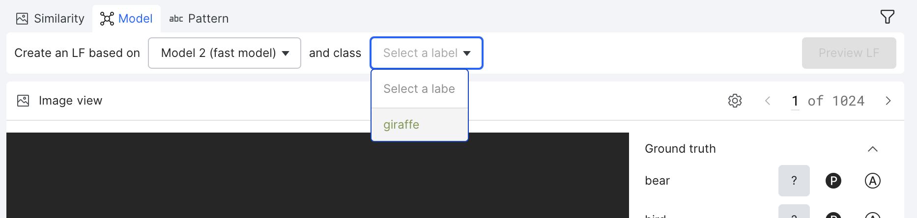
2. Select the Model tab on the LF composer toolbar.
3. Select a pre-trained model and the class that the model was trained on.
4. Click Preview LF.
5. Use the similarity histogram to adjust the thresholds for the images that you would like to label with this LF.
6. Once you are happy with the thresholds that you have selected, click Create LF.

Pattern LFs

The pattern-based LF tool is a native feature in Snorkel Flow that creates LFs based on user-defined rules (e.g., keyword or regex match) against text data that is associated with your images.

To create a pattern-based LF:

1. Select the Pattern tab on the LF composer toolbar.
2. In the textbox, type / to view the list of LF builders that are available.
3. Fill out the required fields on the builder that you selected.
4. Click Preview LF.
5. Use the similarity histogram to adjust the thresholds for the images that you would like to label with this LF.
6. Once you are happy with the thresholds that you have selected, click Create LF.

For more information about creating pattern-based LFs, see Introduction to search based LFs.  For more information about the types of pattern-based LFs that are available, Pattern based LF builders.

Model training

Image Studio supports a fast model variant, which supports the following configurations to train a model at a much faster speed than full models:

• Training on a specific class.
• Training with a training set sample, configured by a negative-to-positive numeric ratio.

Fast models are currently only supported for the logistic regression architecture, and currently only train on the valid data split.

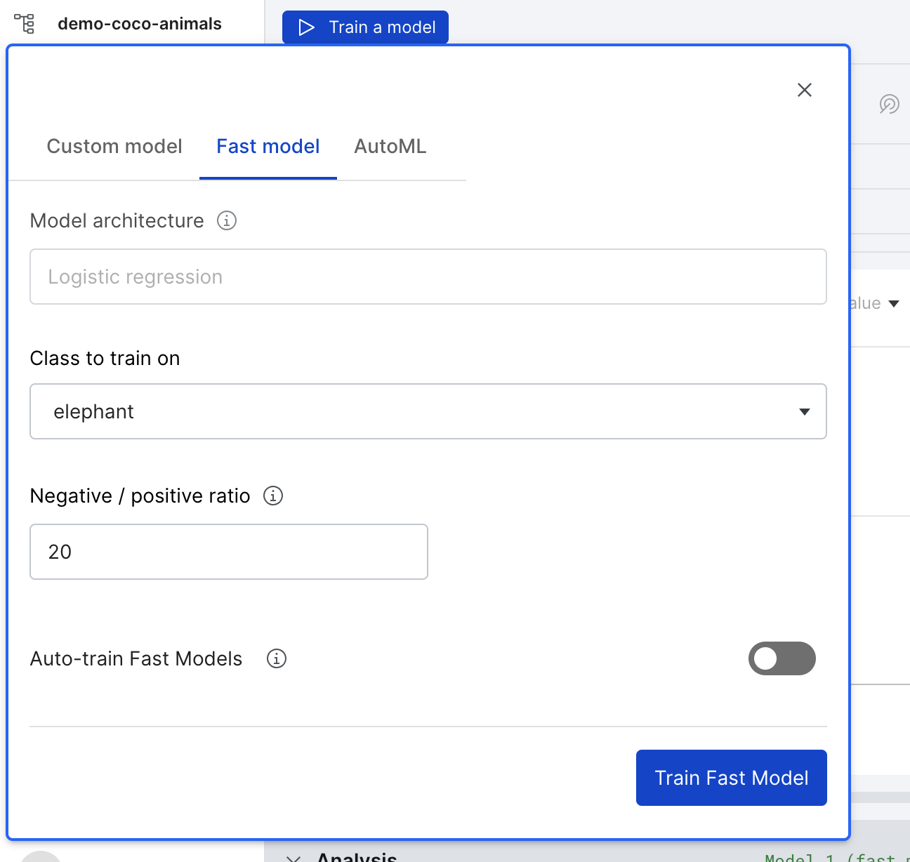
To train a fast model:

1. In the Models pane, click Train a model.
2. Select the Fast model tab.
3. Specify the following options:
   • Class to train on: The specific class for which you would like to train your model.
   • Negative / positive ratio: The negative to positive ground truth sampling ratio to use in the training dataset.
   • Auto-train Fast Models: Turn this on to automatically train a fast model on a sample of your data when your set of active LFs changes.
4. Click Train Fast Model.

While you are waiting for you model to complete, you can continue to explore your data and create LFs.

Once your model is finished running you can view the results in the Models pane and the Analysis pane. Both panes provide charts, metrics and guidance on how to refine your models. For more information about the Models pane, see View and analyze model results. For more information about the Analysis pane, see Analysis: Rinse and repeat.

note

To see model results, you must select the valid split.

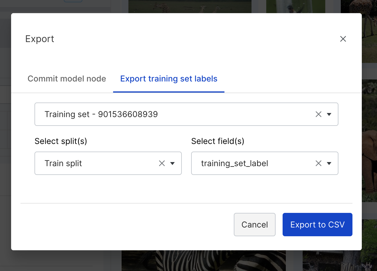
Export labels

At any point you have the option to export your labels to a CSV file:

1. In the top right corner of your screen, click Export.
2. Click Export training set labels.
3. Specify the training set, splits, and fields for which you want to export labels.
4. Click Export to CSV.